
Matplotlib(基礎編)
Contents
Matplotlib(基礎編)#
![]()
まずは、Chainerチュートリアル通りプロット。 簡単なグラフはこれで十分です。
ここでは、numpyでデータを作成しつつプロットを行います。
import numpy as np
import matplotlib.pyplot as plt
numpyの使い方#
一定区間に等間隔で散らばった点を生成
np.arange(開始, 終了, 間隔)
x = np.arange(-1, 1, 0.1)  # -1から1まで、0.1刻みで点を生成する

x
array([-1.00000000e+00, -9.00000000e-01, -8.00000000e-01, -7.00000000e-01,
       -6.00000000e-01, -5.00000000e-01, -4.00000000e-01, -3.00000000e-01,
       -2.00000000e-01, -1.00000000e-01, -2.22044605e-16,  1.00000000e-01,
        2.00000000e-01,  3.00000000e-01,  4.00000000e-01,  5.00000000e-01,
        6.00000000e-01,  7.00000000e-01,  8.00000000e-01,  9.00000000e-01])
関数にわたす
np.arrayを関数に渡すと、その要素全てに同じ操作が加えられます。
例)
np.array([1, 2, 3]) ** 2

# array([1, 4, 9])
その他、numpyで定義されている関数
sincostanlogexp
も使えます。
y = np.sin(x)  # 生成した点をsin関数に渡す

y
array([-8.41470985e-01, -7.83326910e-01, -7.17356091e-01, -6.44217687e-01,
       -5.64642473e-01, -4.79425539e-01, -3.89418342e-01, -2.95520207e-01,
       -1.98669331e-01, -9.98334166e-02, -2.22044605e-16,  9.98334166e-02,
        1.98669331e-01,  2.95520207e-01,  3.89418342e-01,  4.79425539e-01,
        5.64642473e-01,  6.44217687e-01,  7.17356091e-01,  7.83326910e-01])
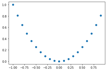
散布図#
plt.scatter(xの配列, yの配列)
平面状に点を打ちます。
x = np.arange(-1, 1, 0.1)
y = x ** 2

plt.scatter(x, y)
<matplotlib.collections.PathCollection at 0x10832fe50>
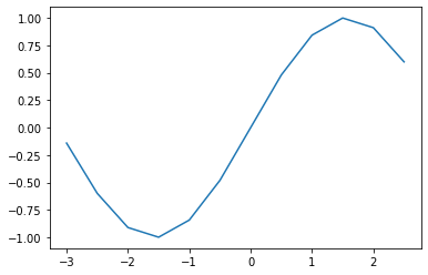
折れ線グラフ#
plt.plot(xの配列, yの配列)
散布図と異なり、隣り合った点をつなげます。
x = np.arange(-3, 3, 0.5)
y = np.sin(x)

plt.plot(x, y)
[<matplotlib.lines.Line2D at 0x108472b00>]
ヒストグラム#
データの生成
\(1〜6\) までの数字をランダムに \(1000\) 回選んで平均を求めます。
これを \(1000\) 回繰り返して、どんな分布になっているかをみてみます。
from random import randint

data = []

for i in range(1000):

    # 1~6までの数字をランダムに選んで足す x 1000回
    sum_of_dice = 0
    for j in range(1000):
        sum_of_dice += randint(1, 6)

    ave_of_dice = sum_of_dice / 1000  # 1000で割って平均を出す
    data.append(ave_of_dice)


print(data[:10])  # 10個目までを見る
[3.517, 3.437, 3.424, 3.409, 3.569, 3.421, 3.517, 3.541, 3.386, 3.412]
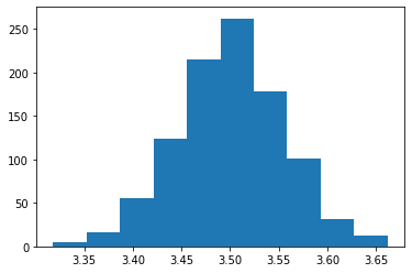
ヒストグラムを作成
plt.hist(データ)
自動的に階級の幅を決めてプロットしてくれます。 この場合は \(10\) 個の階級に分けられていました。
plt.hist(data)
(array([  5.,  16.,  55., 124., 215., 262., 178., 101.,  32.,  12.]),
 array([3.318 , 3.3524, 3.3868, 3.4212, 3.4556, 3.49  , 3.5244, 3.5588,
        3.5932, 3.6276, 3.662 ]),
 <BarContainer object of 10 artists>)
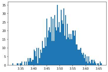
パラメータの調整#
hist関数にオプションで bins=100 を渡すと、階級を \(100\) 個に分けることができます。
plt.hist(data, bins=100)
(array([ 1.,  0.,  0.,  0.,  0.,  1.,  1.,  0.,  1.,  1.,  2.,  0.,  0.,
         2.,  0.,  2.,  0.,  4.,  2.,  4.,  4.,  2.,  3.,  3.,  9.,  8.,
         5., 10.,  1., 10.,  4.,  9.,  7., 14., 10., 10., 16., 11., 27.,
        16., 20., 22., 19., 28., 14., 27., 14., 29., 22., 20., 35., 22.,
        25., 19., 32., 26., 24., 33., 17., 29., 15., 24., 16., 18., 15.,
        18., 15., 20., 20., 17., 20., 12., 12.,  9.,  9.,  9., 10.,  7.,
         6.,  7.,  4.,  6.,  2.,  5.,  1.,  5.,  2.,  1.,  3.,  3.,  1.,
         3.,  2.,  1.,  0.,  1.,  1.,  0.,  2.,  1.]),
 array([3.318  , 3.32144, 3.32488, 3.32832, 3.33176, 3.3352 , 3.33864,
        3.34208, 3.34552, 3.34896, 3.3524 , 3.35584, 3.35928, 3.36272,
        3.36616, 3.3696 , 3.37304, 3.37648, 3.37992, 3.38336, 3.3868 ,
        3.39024, 3.39368, 3.39712, 3.40056, 3.404  , 3.40744, 3.41088,
        3.41432, 3.41776, 3.4212 , 3.42464, 3.42808, 3.43152, 3.43496,
        3.4384 , 3.44184, 3.44528, 3.44872, 3.45216, 3.4556 , 3.45904,
        3.46248, 3.46592, 3.46936, 3.4728 , 3.47624, 3.47968, 3.48312,
        3.48656, 3.49   , 3.49344, 3.49688, 3.50032, 3.50376, 3.5072 ,
        3.51064, 3.51408, 3.51752, 3.52096, 3.5244 , 3.52784, 3.53128,
        3.53472, 3.53816, 3.5416 , 3.54504, 3.54848, 3.55192, 3.55536,
        3.5588 , 3.56224, 3.56568, 3.56912, 3.57256, 3.576  , 3.57944,
        3.58288, 3.58632, 3.58976, 3.5932 , 3.59664, 3.60008, 3.60352,
        3.60696, 3.6104 , 3.61384, 3.61728, 3.62072, 3.62416, 3.6276 ,
        3.63104, 3.63448, 3.63792, 3.64136, 3.6448 , 3.64824, 3.65168,
        3.65512, 3.65856, 3.662  ]),
 <BarContainer object of 100 artists>)
箱ひげ図#
データの生成
確率90%、60%、30%で表が出るコインを用意して、何回連続で表が出るかを調べます。
それぞれ1000回ずつ試行します。
from random import randint
prob_90 = []
prob_60 = []
prob_30 = []

for i in range(1000):

    # 90%が何回連続で出るか
    count_90 = 0
    while randint(1, 100) <= 90:
        count_90 += 1
    prob_90.append(count_90)

    # 60%が何回連続で出るか
    count_60 = 0
    while randint(1, 100) <= 60:
        count_60 += 1
    prob_60.append(count_60)

    # 30%が何回連続で出るか
    count_30 = 0
    while randint(1, 100) <= 30:
        count_30 += 1
    prob_30.append(count_30)

print("90%: ", prob_90[:20])
print("60%: ", prob_60[:20])
print("30%: ", prob_30[:20])
90%:  [5, 9, 17, 3, 11, 1, 12, 1, 7, 17, 10, 5, 0, 7, 7, 0, 24, 10, 1, 1]
60%:  [3, 0, 0, 0, 1, 2, 8, 0, 4, 1, 2, 2, 1, 1, 1, 0, 0, 4, 2, 0]
30%:  [0, 0, 0, 0, 1, 0, 0, 1, 0, 0, 1, 1, 0, 0, 0, 1, 0, 0, 0, 1]
plt.boxplot((prob_90, prob_60, prob_30))
{'whiskers': [<matplotlib.lines.Line2D at 0x10a39fa90>,
  <matplotlib.lines.Line2D at 0x10a39fd60>,
  <matplotlib.lines.Line2D at 0x10a3c0eb0>,
  <matplotlib.lines.Line2D at 0x10a3c1180>,
  <matplotlib.lines.Line2D at 0x10a3c2260>,
  <matplotlib.lines.Line2D at 0x10a3c2530>],
 'caps': [<matplotlib.lines.Line2D at 0x10a3c00a0>,
  <matplotlib.lines.Line2D at 0x10a3c0370>,
  <matplotlib.lines.Line2D at 0x10a3c1450>,
  <matplotlib.lines.Line2D at 0x10a3c1720>,
  <matplotlib.lines.Line2D at 0x10a3c2800>,
  <matplotlib.lines.Line2D at 0x10a3c2ad0>],
 'boxes': [<matplotlib.lines.Line2D at 0x10a39f760>,
  <matplotlib.lines.Line2D at 0x10a3c0be0>,
  <matplotlib.lines.Line2D at 0x10a3c1f90>],
 'medians': [<matplotlib.lines.Line2D at 0x10a3c0640>,
  <matplotlib.lines.Line2D at 0x10a3c19f0>,
  <matplotlib.lines.Line2D at 0x10a3c2da0>],
 'fliers': [<matplotlib.lines.Line2D at 0x10a3c0910>,
  <matplotlib.lines.Line2D at 0x10a3c1cc0>,
  <matplotlib.lines.Line2D at 0x10a3c3070>],
 'means': []}
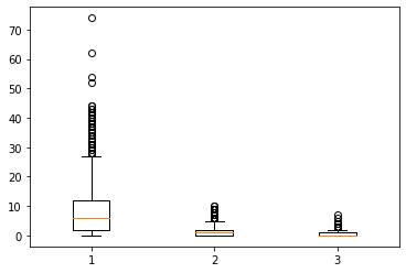
90%だと70回以上出ることもあるのに対して、 30%だと10回以上連続で出ることはほとんどないですね。